Chapter Roadmap
🧭PRODUCTION & RETURNS
COST OF PRODUCTION (Short & Long Run)
FIRM'S REVENUES
FOUR MARKET MODELS
GLOBALIZATION
Theme: this chapter turns from consumer behaviour to producer/firm behaviour. A firm combines factors of production to make output (production function), incurs cost doing so, earns revenue by selling it, and its profit-maximizing price/output decision (MC=MR) differs across four market structures – perfect competition, monopoly, monopolistic competition and oligopoly.
Key Definitions
📘Production Function
Technical relationship between inputs and output: Q = f(L,K) – the maximum output producible from given inputs.
Total Product (TP)
Total amount of goods/services produced using all available inputs in a given period.
Average Product (AP)
Output produced on average per unit of an input: APL=Q/L, APK=Q/K.
Marginal Product (MP)
Change in TP from one extra unit of input: MPL=ΔQ/ΔL – the slope of the TP curve.
Short Run
Time period in which at least ONE input factor is fixed (usually capital/plant) while others are variable.
Long Run
Time period in which NONE of the input factors are fixed – all can be altered.
Law of Variable Proportions
Increasing one variable factor (L) while holding another (K) fixed will eventually cause that factor's marginal product to decline.
Returns to Scale
Relationship between output and a proportionate change in ALL inputs together (long run); contrast with returns to factor/variable proportions (one input, short run).
Short Run vs Long Run – Don't Confuse!
⚖️| Short Run | Long Run | |
|---|---|---|
| Fixed factors | At least one (e.g. plant, building) | None – all factors variable |
| Governing law | Law of Variable Proportions (returns to factor) | Returns to Scale |
| Adjustment | Only variable inputs (labour, material) can change | Even plant size/structure can change |
| Cost curves | TFC, TVC, TC, AFC, AVC, ATC, MC all relevant | No fixed cost gap – only ATC (=AVC) relevant |
Law of Variable Proportions – 3 Stages of Production
📜| Stage | Name | What Happens |
|---|---|---|
| I | Increasing Returns | Each extra worker's contribution > previous one's – MP and TP both rise |
| II | Diminishing Returns | MP falls after a point (but stays positive) – TP still rises, but at a decreasing rate |
| III | Negative Returns | MP becomes zero then negative – TP starts to FALL |
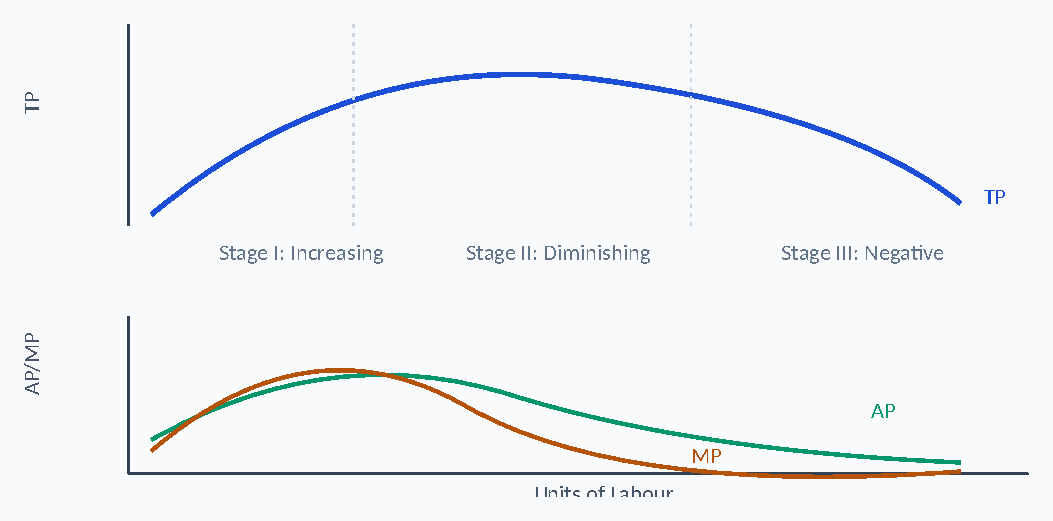
MP and AP curves intersect where AP is at its MAXIMUM. When MP=0, TP is at its MAXIMUM.
Worked Example: Returns to Factor
🧪| Labour (L) | 0 | 1 | 2 | 3 | 4 | 5 | 6 | 7 |
|---|---|---|---|---|---|---|---|---|
| TP (K fixed=10) | 0 | 5 | 15 | 30 | 40 | 45 | 45 | 40 |
| MP | – | 5 | 10 | 15 | 10 | 5 | 0 | −5 |
MP rises through L=3 (Stage I), falls but stays positive through L=5 (Stage II), hits 0 at L=6 and turns negative at L=7 (Stage III).
Returns to Scale (Long Run)
📌INCREASING RETURNS TO SCALE
- Output rises MORE than proportionately to inputs (economies from bigger, better-managed operations)
CONSTANT RETURNS TO SCALE
- Output rises IN PROPORTION to inputs (e.g. doubling inputs exactly doubles output)
DIMINISHING RETURNS TO SCALE
- Output rises LESS than proportionately (rare) – rising admin/coordination cost
| Scale (Labour+Land) | Total Returns | Marginal Returns | Stage |
|---|---|---|---|
| 1L+2 acres | 4 | 4 | Increasing |
| 2L+4 acres | 10 | 6 | Increasing |
| 4L+8 acres | 28 | 10 | Constant (starts) |
| 6L+12 acres | 48 | 10 | Constant |
| 7L+14 acres | 56 | 8 | Decreasing |
| 8L+16 acres | 62 | 6 | Decreasing |
Cost of Production – Explicit vs Implicit Cost
⚖️TOTAL ECONOMIC COST
Total Economic Cost = Explicit Cost + Implicit Cost
Explicit = out-of-pocket cash cost (wages, rent, materials) | Implicit = opportunity cost of owner's own resources (e.g. forgone salary)
Short-run Cost Formulas
🧮TOTALS
- TC = TFC + TVC
- Fixed cost: unchanged with output. Variable cost: changes with output.
AVERAGES & MARGINAL
- AFC = TFC ÷ Q | AVC = TVC ÷ Q | ATC = TC ÷ Q = AFC + AVC
- MC = ΔTC ÷ ΔQ (slope of TC curve)
MC & AC Relationship
📌MC < AC
AC is FALLING (extra unit costs less than average)
MC = AC
AC is at its MINIMUM (most efficient point)
MC > AC
AC is RISING (extra unit costs more than average)
Exam clue: MC always cuts AC (and AVC) at AC's (AVC's) MINIMUM point – this mirrors how MP cuts AP at AP's maximum (productivity and cost curves move inversely to each other).
Cost Curves – Graph
📈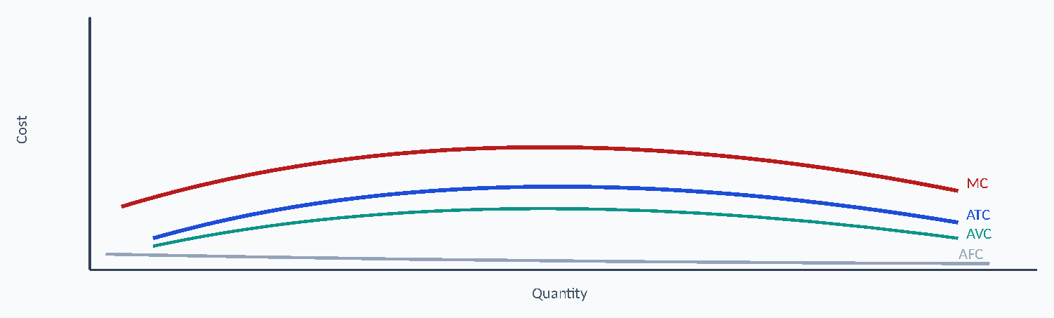
MC dips below then cuts ATC and AVC at their minimum points; AFC continually falls (spread over more units) as Q rises, so the gap between ATC and AVC narrows with output.
Cost of Production in Long Run
💰In the long run there is no fixed cost, so TC = TVC and only ATC (Long-Run ATC) matters – it is the envelope of many short-run ATC curves as the firm moves between plant sizes.
Economies vs Diseconomies of Scale
⚖️ECONOMIES OF SCALE (LRATC ↓ AS OUTPUT ↑)
- Specialization of labour
- Technological/specialized equipment
- Bulk-buying discounts
- Cheaper cost of capital (better bargaining with banks)
- Shared repair & maintenance facilities
- Start-up costs spread over more output
- Advertising cost spread over more output
DISECONOMIES OF SCALE (LRATC ↑ AS OUTPUT ↑)
- Costly coordination among units
- Management hierarchy slows decisions
- Staff overheads grow disproportionately
- Labour unrest/industrial disputes
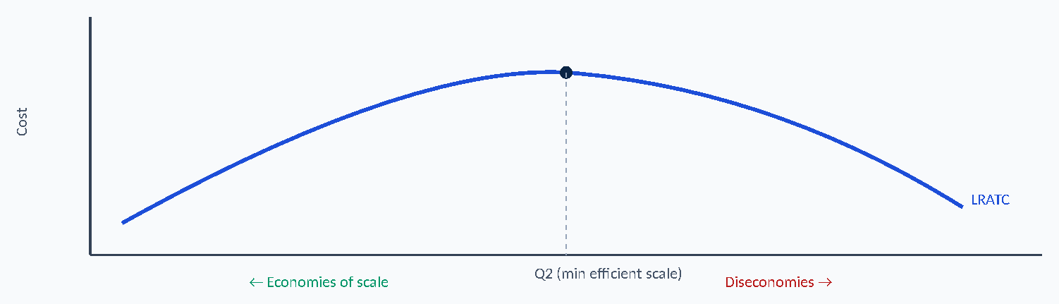
As output expands from Q1 to Q2, ATC falls from C1 to C2 (economies of scale). Beyond Q2, economies are exhausted and ATC starts RISING (diseconomies of scale).
Firm's Revenues – Formulas
🧮TOTAL, AVERAGE & MARGINAL REVENUE
TR = P × Q | AR = TR ÷ Q = P | MR = ΔTR ÷ ΔQ
AR always equals Price – true in every market structure
Profit Rule & Profit/loss Test
📌PROFIT MAXIMIZATION RULE
- Necessary condition: MC = MR
- Sufficient condition: MC = MR while MC is RISING
PROFIT = TR − TC
- TR > TC → Profit
- TR < TC → Loss
- TR = TC → Break-even
The Four Market Models – Overview
📌| Perfect Competition | Monopoly | Monopolistic Competition | Oligopoly | |
|---|---|---|---|---|
| No. of firms | Very large | One (single seller) | Large number | Few (2–20) |
| Product | Homogeneous | Unique, no substitutes | Differentiated | Homogeneous or differentiated |
| Entry barriers | None (free entry/exit) | Very heavy | Few | Heavy |
| Price control | Price taker (P=AR=MR) | Price maker (P>MR) | Some control (P>MR) | Interdependent pricing |
| Long-run profit | Normal profit only | Super-normal possible | Normal profit only | Super-normal possible |
Perfect Competition – Characteristics
📌PRECONDITIONS
- Large number of buyers & sellers – none can influence price
- Homogeneous product – no differentiation
- Free entry and exit
- Perfect knowledge of prices
- No transport cost, perfect factor mobility
- Firms are PRICE TAKERS – P = AR = MR (flat demand curve)
Perfect Competition – Profit/loss Scenarios (Short Run)
📌| Scenario | Condition (at MC=MR) | Meaning |
|---|---|---|
| Super-normal (abnormal) profit | P > ATC | Revenue exceeds normal profit – extra/excess profit |
| Normal profit | P = ATC | TR = Explicit + Implicit cost – just enough to keep firm in industry |
| Sub-normal profit (normal loss) | AVC < P < ATC | Covers variable cost + part of fixed cost – firm stays open |
| Shut-down point (abnormal loss) | P < AVC | Can't even cover variable cost – firm should shut down |
Shut-down rule: a firm continues to produce in the short run as long as P ≥ AVC (fixed costs are sunk and must be paid either way); it only shuts down when P falls below AVC.
Accounting Profit vs Economic Profit
⚖️PROFIT FORMULAS
Accounting Profit = TR − Explicit Cost | Economic Profit = TR − (Explicit + Implicit Cost)
Economic (Normal) profit also accounts for the OPPORTUNITY COST of the owner's own resources (e.g. forgone salary)
Worked example: Zain's law firm – Revenue Rs.200,000; Explicit costs (rent Rs.50,000 + staff Rs.35,000) = Rs.85,000 ⇒ Accounting profit = Rs.115,000. But he forgoes a Rs.125,000 salary (implicit cost) ⇒ Economic profit = 200,000 − (85,000+125,000) = −Rs.10,000 (an economic LOSS, even though accounting profit is positive).
Short Run vs Long Run Under Perfect Competition
⚖️Existing firms earn super-normal profit
New firms attracted & enter (free entry)
Supply ↑, price ↓ until only NORMAL profit remains
Existing firms make losses
Weak firms exit the industry
Supply ↓, price ↑ until remaining firms earn NORMAL profit
Conclusion: in the long run, perfectly competitive firms earn only NORMAL profit – entry eliminates economic (super-normal) profit, exit eliminates loss.
Monopoly – Characteristics & Barriers
📌CHARACTERISTICS
- Single seller – firm behaves like the whole industry
- Heavy barriers to entry
- No close substitutes
- PRICE MAKER: downward-sloping demand curve, AR=P>MR
BARRIERS TO ENTRY
- Control over key inputs
- Structural barriers / economies of scale (natural monopoly)
- Cost advantages / predatory (dumping) pricing
- Regulatory & legal barriers (patents, licences)
Examples from the text: SSGC/SNGPL (gas), WAPDA (power), PTCL (telecom) – Pakistani natural/regulated monopolies.
Monopoly Revenue Behaviour
💰As a monopolist cuts price to sell more, TR rises then falls; MR falls faster than AR (price) and can turn negative. TR is maximized where MR = 0.
Exam clue: Under monopoly, MR < AR (=Price) always – unlike perfect competition where MR = AR = P.
Monopoly: Advantages vs Disadvantages
⚖️| Arguments FOR Monopoly | Arguments AGAINST Monopoly |
|---|---|
| Price stability (no competitive fluctuation) | Higher prices than competitive markets |
| Benefits from economies of scale (natural monopoly) | Loss of consumer surplus |
| Super-normal profits can fund R&D | Little incentive to innovate (organizational slack) |
| Able to take a long-term investment approach | Possible large-scale diseconomies / X-inefficiency |
| Source of essential public utilities | Price discrimination; inferior quality product possible |
Price Discrimination
📌PRE-CONDITIONS
- Firm must be a price maker
- Market must be segregable (by income, elasticity, etc.)
- Resale must be preventable
Examples: peak/off-peak electricity rates, weekend vs weekday movie prices, bulk-buy discounts, off-season price cuts.
Monopolistic Competition – Characteristics
📌A BLEND OF MONOPOLY + PERFECT COMPETITION
- Large number of firms, each with a small market share
- Differentiated products (brand identity)
- Few barriers to entry/exit
- High brand loyalty
- Non-price competition (advertising, service, design)
- Demand curve: downward-sloping but relatively ELASTIC (close substitutes exist)
Examples: restaurants, shoe outlets, hair salons/beauty parlours, hand-wash brands – each has its own loyal customer base within a competitive category.
Monopolistic Competition – Short Run vs Long Run
⚖️| Period | Condition (at MC=MR) | Outcome |
|---|---|---|
| Short Run | AR > ATC | Super-normal profit possible (like a mini-monopoly) |
| Long Run | AR = ATC (P = ATC) | Free entry erodes extra profit – only NORMAL profit remains |
Monopolistic Competition: Advantages vs Disadvantages
⚖️| Advantages | Disadvantages |
|---|---|
| No significant entry barriers – contestable market | Differentiation can be artificial/unnecessary |
| Differentiation increases consumer choice | Wasteful competitive advertising spend |
| More efficient than monopoly | Higher cost than perfect competition |
| Heavy advertising = more informed consumers |
Oligopoly – Characteristics
📌KEY FEATURES
- Few sellers (2–20), high concentration ratio
- Interdependence of firms – each firm's move affects rivals
- Heavy advertising, heavy entry barriers
- Indeterminate demand curve (rival reactions unpredictable)
- Homogeneous or differentiated products
Examples: media, automobiles, airlines, cellular services, beverages.
Types of Oligopoly – Classification
🧩OLIGOPOLY MODELS
Collusive Oligopoly (Price Cartel)
Firms formally/informally agree on price & output (e.g. OPEC). Needs: few known firms, similar cost/product, dominant firm, stable market, no govt. interference. Rare in practice.
Non-Collusive Oligopoly (Kinked Demand Curve)
No agreement; each firm independent. Rivals MATCH price cuts but IGNORE price rises → a "kinked" demand curve at the ruling price P*.
Kinked Demand Curve – Decision Tree
📈FIRM RAISES PRICE above P*?
FIRM CUTS PRICE below P*?
Rivals IGNORE it → firm loses many customers → demand ELASTIC above P*
Rivals MATCH the cut → little gain in sales → demand INELASTIC below P*
This creates a "kink" at price P*, quantity Q*, and a discontinuous MR curve – explaining why oligopoly prices tend to stay STABLE even when costs change moderately.
Price Cartel: Harms to Society
📌- Higher prices (super profits at buyers' expense)
- Lack of transparency (hidden charges/info)
- Restricted output to inflate price
- Poor quality goods (no incentive to improve)
Globalization & Firm's Behaviour
📌BENEFITS OF GLOBALIZATION
- Division of labour & specialization
- Economies of scale from larger markets
- Increased competition (erodes monopolies)
- Higher productivity via modern technology
- Greater availability of capital
COSTS OF GLOBALIZATION
- Damaging for infant industries
- Structural unemployment
- Environmental concerns
- Trade imbalances
- Inflation risk
Exam Patterns & MCQ Quick Clues
🎯"MC = MR, and MC rising"
Profit-maximizing output (sufficient condition)
"Price maker, downward AR, no substitutes"
Monopoly
"Many firms, differentiated product, non-price competition"
Monopolistic Competition
"Few firms, interdependent, kinked demand"
Oligopoly (non-collusive)
"P < AVC"
Shut-down point (short run)
"Forgone salary/rent used in own business"
Implicit cost
⚠ ECONOMICS EXAM TRAPS
Trap: Confusing returns to a FACTOR (one input varies, short run) with returns to SCALE (all inputs vary, long run) – different laws, different assumptions.
Trap: Forgetting implicit cost when computing economic profit – accounting profit can be positive while economic profit is negative.
Trap: Assuming MR=AR in every market – only true under PERFECT COMPETITION; under monopoly/imperfect competition MR < AR.
Trap: Mixing up shut-down (P<AVC) with sub-normal profit (AVC<P<ATC) – only the former means the firm should stop producing NOW.
Trap: Believing all 4 market structures earn only normal profit long run – only Perfect Competition AND Monopolistic Competition do; Monopoly and Oligopoly can retain super-normal profit due to entry barriers.
Complete Chapter Decision Tree
📌QUESTION GIVEN → Production/cost/revenue/market-structure question? → Short run or long run? → Identify the relevant formula (TP/AP/MP, TC/AC/MC, TR/AR/MR) → Which market structure applies (check characteristics)? → Apply MC=MR rule → Compare P to ATC/AVC for profit/loss position → Interpret & select final answer
PRC-3 ECONOMICS – CHAPTER 4 IN 60 SECONDS
- Production function: Q=f(L,K); TP, AP=Q/input, MP=ΔQ/Δinput.
- Law of variable proportions: MP eventually falls as one input rises (short run).
- Returns to scale: long-run response of output to ALL inputs changing together.
- Cost: TC=TFC+TVC; MC=AC's minimum-cutting curve.
- Economies of scale: LRATC falls; Diseconomies: LRATC rises.
- Revenue: TR=PxQ; AR=P always; MR=ΔTR/ΔQ.
- Profit rule: MC=MR (necessary); MC rising at that point (sufficient).
- Perfect competition: price taker, P=AR=MR, normal profit long run.
- Monopoly: price maker, MR<AR, super-normal profit possible long run.
- Monopolistic competition: many firms, differentiated, normal profit long run.
- Oligopoly: few firms, interdependent, kinked demand (non-collusive) or cartel (collusive).
Chapter Memory Map
🧠Preparing for ICAP PRC-3?
Join Learning League for chapter-wise classes, practice MCQs and tests on our student portal. Message us on WhatsApp to enrol.