Chapter Roadmap
🧭ELASTICITY OF DEMAND
(PED & measurement methods)
OTHER ELASTICITIES (Income & Cross)
DETERMINANTS & APPLICATIONS
ELASTICITY OF SUPPLY & TIME
Theme: the law of demand tells us direction (price↑ ⇒ Qd↓) but not magnitude. Elasticity measures HOW MUCH quantity responds to a change in price, income, or the price of another good – this drives real business decisions on pricing, taxation, and trade.
Key Definitions
📘Elasticity of Demand (PED)
Degree of responsiveness of quantity demanded to a change in the good's own price.
Elastic Demand
% change in Qd > % change in price – demand is sensitive to price.
Inelastic Demand
% change in Qd < % change in price – demand is insensitive to price.
Unit Elastic Demand
% change in Qd = % change in price – total revenue stays unchanged.
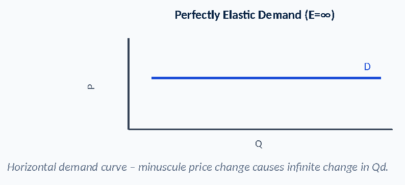
Perfectly Elastic (E=∞)
Smallest price change causes an infinitely large change in demand – horizontal demand curve.
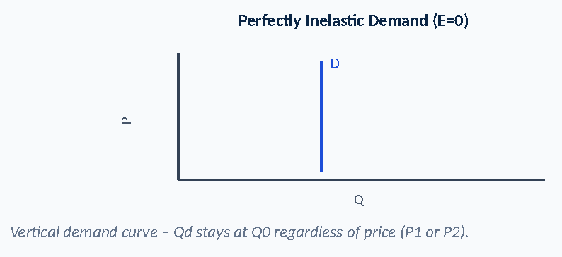
Perfectly Inelastic (E=0)
Demand totally unaffected by price change – vertical demand curve.
Income Elasticity of Demand
Responsiveness of Qd to a change in consumer income; positive for normal goods, negative for inferior goods.
Cross Elasticity of Demand
Responsiveness of Qd for good A to a change in the price of good B; positive = substitutes, negative = complements.
Degrees of Elasticity & Effect on Revenue
🔁| Coefficient | Degree | Effect of a Price FALL on Total Revenue |
|---|---|---|
| E = 0 | Perfectly inelastic | Qd unaffected – revenue falls in same proportion as price |
| 0 < E < 1 | Relatively inelastic | Revenue FALLS (Qd rise fails to offset price fall) |
| E = 1 | Unit elastic | Revenue UNCHANGED (offsetting effects exactly cancel) |
| E > 1 | Relatively elastic | Revenue RISES (Qd rise more than offsets price fall) |
| E = ∞ | Perfectly elastic | Infinitely responsive – any price rise takes Qd to zero |
Exam clue: Elastic → Price and Revenue move in OPPOSITE directions. Inelastic → Price and Revenue move in the SAME direction. Unit elastic → Revenue does not change with price.
Method 1: Total Expenditure (Total Revenue) Method
💰RULE (ALFRED MARSHALL)
- Total expenditure ↑ when price falls → demand is relatively elastic
- Total expenditure ↓ when price falls → demand is relatively inelastic
- Total expenditure unchanged when price falls → demand is unit elastic
| Case | Price (Rs.) | Qty (litres) | Total Expenditure | Result |
|---|---|---|---|---|
| Inelastic (η<1) | 200 → 400 | 30 → 25 | 6,000 → 10,000 (↑) | Expenditure rises with price → Inelastic |
| Elastic (η>1) | 200 → 400 | 30 → 10 | 6,000 → 4,000 (↓) | Expenditure falls with price rise → Elastic |
| Unit elastic (η=1) | 200 → 400 | 30 → 15 | 6,000 → 6,000 (no change) | Expenditure constant → Unit elastic |
Method 2: Percentage (Proportionate) Method
🛠PRICE ELASTICITY OF DEMAND
η = [(Q₂−Q₁)÷((Q₂+Q₁)/2)] ÷ [(P₂−P₁)÷((P₂+P₁)/2)]
Uses AVERAGE price & quantity so η is the same moving either direction along the curve | Take the ABSOLUTE value to compare against 1
ELASTIC EXAMPLE
- Qd: 30→10, P: 200→400
- η = −1.5 → |1.5| > 1 – Elastic
INELASTIC EXAMPLE
- Qd: 30→25, P: 200→400
- η = −0.27 → |0.27| < 1 – Inelastic
UNIT ELASTIC EXAMPLE
- Qd: 30→15, P: 200→400
- η = −1 → |1| = 1 – Unit elastic
Point Elasticity vs Arc Elasticity
⚖️| Point Elasticity | Arc Elasticity | |
|---|---|---|
| When used | Very small/nominal price change (e.g. petroleum) | Significant/large price change (e.g. poultry, dairy, crops) |
| Formula | η = (ΔQ/Q₀) ÷ (ΔP/P₀) | η = [(Q₁−Q₀)/(Q₁+Q₀)] × [(P₁+P₀)/(P₁−P₀)] |
| Worked example | P: 12→11.75, Q: 100→101 ⇒ η = −0.48 (Inelastic) | P: 8→12, Q: 300→100 ⇒ η = −2.5 (Elastic) |
Method 3: Geometric Method
🛠Measures elasticity at any point on a straight-line demand curve using: η = Lower part of the demand curve (below the point) ÷ Upper part of the demand curve (above the point).
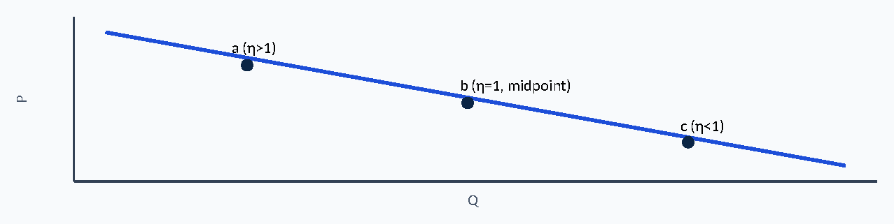
Along a straight-line demand curve: points near the TOP (price-axis end) are elastic (η>1); the MIDPOINT is unit elastic (η=1); points near the BOTTOM (quantity-axis end) are inelastic (η<1).
Two Extremes of Price Elasticity of Demand
📌
Income Elasticity of Demand (YED)
📌INCOME ELASTICITY OF DEMAND
η = % change in Qd ÷ % change in Income = (ΔD/D) ÷ (ΔI/I)
Positive coefficient = Normal good | Negative coefficient = Inferior good
NORMAL GOODS (YED > 0)
- Qd rises as income rises
- Superior/luxury goods: Qd rises MORE than proportionately (e.g. luxury cars – elastic)
- Necessities: Qd rises but inelastically
INFERIOR GOODS (YED < 0)
- Qd FALLS as income rises – consumers switch to superior alternatives
- Examples: inexpensive/frozen food, long-route bus tickets, reconditioned cars
Worked example: Income Rs.10,000→15,000 (+40%); Demand 50→40 units (−22.2%) ⇒ YED = −22.2% ÷ 40% = −0.56 ⇒ Negative & |value|<1 ⇒ Inferior good, income-inelastic.
Applied use: products with HIGH income elasticity get hit hardest during a recession (e.g. cars fell more than food demand during COVID-19); firms use YED to plan future product ranges as incomes grow.
Cross Elasticity of Demand (XED)
📌CROSS ELASTICITY OF DEMAND FOR GOOD A W.R.T. PRICE OF GOOD B
Ec = (ΔQa ÷ Qa) ÷ (ΔPb ÷ Pb)
Unlike PED, the coefficient can be POSITIVE or NEGATIVE
| Sign of Ec | Relationship | Example |
|---|---|---|
| Positive | Substitutes – demand for A moves SAME direction as price of B | Lipton tea price ↑ → demand for Supreme tea ↑ (Ec = +3.01, elastic) |
| Negative | Complements – demand for A moves OPPOSITE direction to price of B | Shoe price ↑ → demand for shoelaces ↓ (Ec = −3.01, elastic) |
| Zero / near zero | Independent (unrelated) goods – no relationship | Price of butter has no effect on demand for notebooks |
Larger positive coefficient = closer substitutes; larger negative coefficient = stronger complementarity.
Determinants of Elasticity of Demand
📌Close substitutes available
Demand MORE elastic
Complementary good's price rises
Demand for THIS good MORE inelastic
Good is a necessity
Demand MORE inelastic (luxuries → more elastic)
Strong brand loyalty/habit
Demand MORE inelastic
Small % of income spent on good
Demand MORE inelastic
Longer time period allowed
Demand becomes MORE elastic (time to adjust/switch)
Applications of Elasticity of Demand
📌PRICE DETERMINATION
- Elastic goods: keep price low (else lose sales to substitutes)
- Inelastic goods: price can be high (necessities)
TAXATION (FINANCE MINISTER)
- Tax inelastic goods (tobacco, electricity) → high revenue
- Tax on elastic goods → demand falls sharply, revenue falls
MONOPOLIST'S GUIDANCE
- Inelastic goods: high price, low quantity
- Elastic goods: low price + promos to keep buyers
TRANSPORT FARES
- Elastic transport (bus/taxi): fares kept LOW
- Inelastic transport (airways, no alternative): fares HIGH
BALANCE OF TRADE
- Elastic export demand → low earnings, unfavourable trade balance
- Countries want inelastic demand abroad to raise price & boost exports
RECESSION PLANNING
- High-YED products hit hardest when income falls
- Firms reallocate resources accordingly
Elasticity of Supply (Es)
📌PRICE ELASTICITY OF SUPPLY
Es = [(Q₂−Q₁)÷((Q₂+Q₁)/2)] ÷ [(P₂−P₁)÷((P₂+P₁)/2)]
Direct/positive relationship between price & quantity supplied ⇒ Es is ALWAYS positive
| Case | Price | Quantity | Es | Result |
|---|---|---|---|---|
| Inelastic supply | 100→200 | 50→60 | 0.27 | Es < 1 – Inelastic |
| Elastic supply | 100→200 | 50→150 | 1.5 | Es > 1 – Elastic |
| Unit elastic supply | 100→200 | 50→100 | 1.0 | Es = 1 – Unit elastic |
Geometric Shortcuts for Linear Supply Curves
📈INTERSECTS PRICE AXIS
- Elastic (Es>1) at ALL points
INTERSECTS QUANTITY AXIS
- Inelastic (Es<1) at ALL points
PASSES THROUGH ORIGIN
- Unit elastic (Es=1) at ALL points
These shortcut rules apply only to LINEAR (straight-line) supply curves – not valid for non-linear curves.
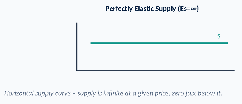
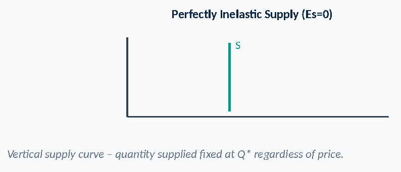
Two Extremes of Supply Elasticity
📌
Determinants of Elasticity of Supply
📌More firms in the industry
Supply MORE elastic
Stocks/inventory available
Supply MORE elastic (can meet demand from stock)
Spare capacity exists
Supply MORE elastic; full capacity → MORE inelastic
Resources easily switched to other goods
Supply MORE elastic
Longer time period allowed
Supply becomes MORE elastic
Elasticity of Supply & Time
📌| Time Period | Ability to Adjust | Elasticity |
|---|---|---|
| Momentary/Immediate market period | Insufficient time to change output at all | Perfectly inelastic |
| Short run | Plant capacity fixed; minor efficiency/technique tweaks only | Relatively inelastic |
| Long run | All adjustments possible (plant size, structure, new capacity) | Highly/relatively elastic |
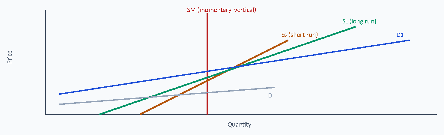
Demand rises from D to D1 at price P0. In the momentary period price jumps to PM (Qty fixed); in the short-run price settles lower at PS as supply adjusts a little; in the long run price falls further to PL as supply becomes fully elastic. Conclusion: the longer the time allowed, the more elastic supply becomes.
Exam Patterns & MCQ Quick Clues
🎯"Price & revenue move in opposite directions"
Elastic demand (E>1)
"Price & revenue move in the same direction"
Inelastic demand (E<1)
"Coefficient is negative"
Inferior good (YED) OR complements (XED)
"Coefficient is positive" (income/related-price context)
Normal good (YED) OR substitutes (XED)
"Nominal/very small price change"
Use Point Elasticity
"Significant/large price change"
Use Arc Elasticity
"Supply curve is vertical / no time to adjust"
Momentary period – perfectly inelastic supply
⚠ ECONOMICS EXAM TRAPS
Trap: Forgetting to take the ABSOLUTE value of PED before comparing to 1 (PED is naturally negative due to the law of demand).
Trap: Confusing YED sign rules (normal=positive/inferior=negative) with XED sign rules (substitutes=positive/complements=negative) – they look similar but classify different things.
Trap: Elasticity of supply coefficient is ALWAYS positive (direct relationship) – unlike PED, never take its negative sign as meaningful.
Trap: Reversing the geometric supply-curve rule – intersecting the PRICE axis is ELASTIC, intersecting the QUANTITY axis is INELASTIC.
Trap: Assuming elasticity of supply is fixed – it INCREASES over time (momentary → short run → long run).
Trap: Mixing up Point Elasticity (small change) with Arc Elasticity (large change) formulas.
Complete Chapter Decision Tree
📌QUESTION GIVEN → Which elasticity is asked (PED / YED / XED / Es)? → Is the price/income change small (point) or large (arc)? → Apply the relevant formula → Calculate & take absolute value where relevant (PED, Es) → Compare to 1 (or check sign for YED/XED) → Interpret (elastic/inelastic/normal/inferior/substitute/complement) → Select final answer
PRC-3 ECONOMICS – CHAPTER 3 IN 60 SECONDS
- PED: %ΔQd ÷ %ΔP; elastic if >1, inelastic if <1, unit if =1.
- TR method: price↓ & TR↑ = elastic; price↓ & TR↓ = inelastic; TR same = unit.
- Point elasticity: tiny price change. Arc elasticity: large price change.
- Geometric method: lower part ÷ upper part of demand curve at a point.
- YED: positive = normal good; negative = inferior good.
- XED: positive = substitutes; negative = complements; ~0 = independent.
- PED determinants: substitutes, necessity/luxury, brand loyalty, % of income, time.
- Es: always positive; rises with more firms, stock, spare capacity, resource mobility, time.
- Linear supply curve: hits price-axis=elastic; hits quantity-axis=inelastic; through origin=unit elastic.
- Time & supply: momentary=perfectly inelastic; short run=relatively inelastic; long run=elastic.
Chapter Memory Map
🧠Preparing for ICAP PRC-3?
Join Learning League for chapter-wise classes, practice MCQs and tests on our student portal. Message us on WhatsApp to enrol.