Chapter Roadmap
🧭MARKET ENVIRONMENT
DEMAND & ITS LAW
SUPPLY & ITS LAW
PRICE DETERMINATION & EQUILIBRIUM
SHIFTS, GOVT POLICY & E-BUSINESS
Theme: markets bring buyers and sellers together. Demand and supply are the two forces that interact to fix price and quantity in a market – understanding how each force behaves (and what shifts it) explains everyday changes in prices, from chicken to room coolers to sugar cane.
Key Definitions
📘Demand
Quantity of a good/service buyers are willing AND able to buy at a given price and time – desire alone (without ability to pay) is not demand.
Law of Demand
Ceteris paribus, as price rises the quantity demanded contracts, and as price falls it extends – an inverse price-quantity relationship.
Supply
Amount of a product offered for sale at a given price and moment – NOT the entire stock held by the producer.
Law of Supply
Ceteris paribus, as price rises the quantity supplied extends, and as price falls it contracts – a direct/positive price-quantity relationship.
Market Demand
Horizontal summation of all individual consumers' demand curves in the market.
Equilibrium
Situation where no agent wants to change decisions and all decisions are compatible – market demand = market supply (Qd = Qs).
Ceteris Paribus
"All other things remaining constant/unchanged" – the key assumption behind both demand and supply laws.
Reservation Price
The lowest price at which a firm is willing to sell a good or provide a service.
Why Demand Slopes Downward – Income & Substitution Effects
🔁INCOME EFFECT
- Price rises → consumer's real purchasing power falls → feels poorer → buys less
SUBSTITUTION EFFECT
- Price rises → good becomes dearer relative to alternatives → consumers switch to substitutes
Assumptions of Law of Demand
📌HELD CONSTANT (CETERIS PARIBUS)
- No change in average income of consumers
- No change in population size
- No change in prices of related goods (substitutes/complements)
- No change in taste, habit, fashion or weather
- No change in future price expectations
- No change in advertisement
Demand Schedule & Curve (Chicken Example)
🧪| Price (Rs./kg) | 500 | 400 | 300 | 200 | 100 |
|---|---|---|---|---|---|
| Quantity Demanded (kg) | 10 | 20 | 35 | 55 | 80 |
As price falls from Rs.500 to Rs.100, quantity demanded rises from 10kg to 80kg – confirming the inverse price-quantity relationship (downward-sloping demand curve D, price on Y-axis, quantity on X-axis).
Movement Along vs Shift of the Demand Curve
📈PRICE OF THE GOOD ITSELF CHANGES?
OTHER DETERMINANT CHANGES? (income, taste, weather, population, related-good prices, ads)
MOVEMENT along the SAME curve → "Extension" (price↓, Qd↑) or "Contraction" (price↑, Qd↓) – also called change in quantity demanded
SHIFT of the WHOLE curve → "Rise in demand" (shift right) or "Fall in demand" (shift left) – also called change in demand
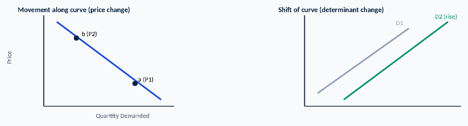
Factors Causing a Shift in Demand – Cause & Effect
🔍Income ↑
Demand for (normal) goods ↑ – curve shifts right
Taste turns favourable
Demand ↑ regardless of price
Weather suits the product (e.g. winter → tea)
Demand for that product ↑
Population ↑
Demand for most goods ↑
Price of a substitute ↑
Demand for THIS good ↑ (buyers switch to it)
Successful advertisement
Demand for that good ↑
Exceptions to the Law of Demand
📜BASIC NECESSITIES
- Sugar, rice, wheat – bought regardless of price change
UNIQUE/DISTINCTIVE GOODS
- Demand rises WITH price for a particular group (status/prestige goods)
CHANGE IN INCOME
- Rising income can raise demand even as price rises
CONSUMER IGNORANCE
- Unaware of cheaper alternatives elsewhere
UNCERTAIN CONDITIONS
- Fear of future shortage → buy more despite high price
Practical importance of Law of Demand: helps in price determination, firm's future planning/decision-making, and assists the Finance Minister in setting tax rates without eroding taxable revenue.
Supply Schedule & Curve (Rice Example)
🧪| Price (Rs./ton) | 10 | 20 | 30 | 40 | 50 | 60 |
|---|---|---|---|---|---|---|
| Quantity Supplied (tons) | 0 | 5 | 15 | 30 | 50 | 65 |
Positive/direct relationship – as price rises, quantity supplied rises. Supply curve S is upward sloping (price on Y-axis, quantity on X-axis).
Assumptions of Law of Supply
📌HELD CONSTANT (CETERIS PARIBUS)
- Cost of production remains constant
- Technology/technique of production unchanged
- No change in taxes or subsidies
- Input/raw material prices unchanged
- Prices of other goods unaffected
Movement Along vs Shift of the Supply Curve
📈PRICE OF THE GOOD ITSELF CHANGES?
OTHER FACTOR CHANGES? (input cost, technology, taxes/subsidies, price of other goods)
MOVEMENT along the SAME curve = change in quantity supplied (extension/contraction)
SHIFT of the WHOLE curve = change in supply (rise = right, fall = left)
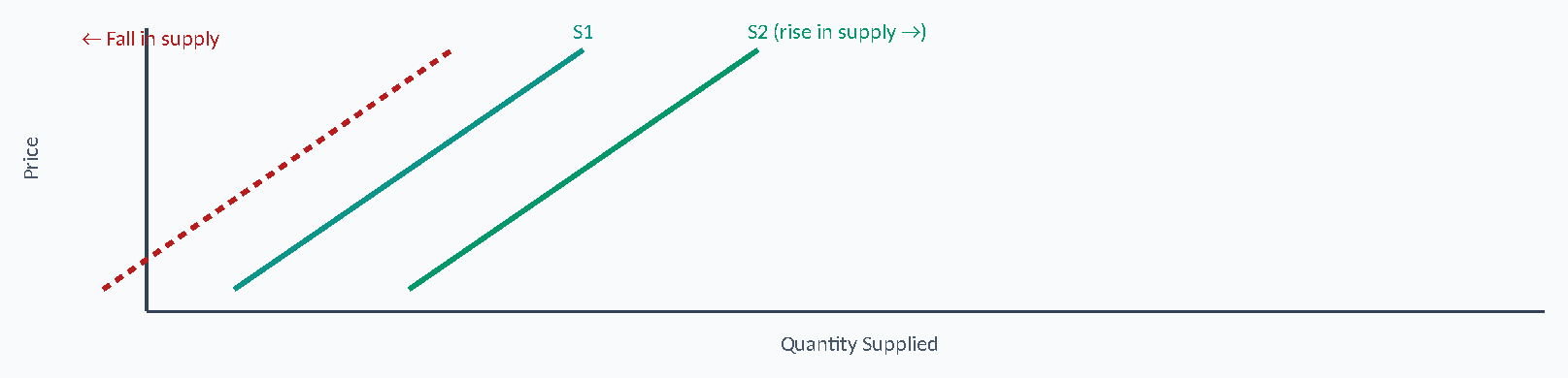
Factors Causing a Shift in Supply – Cause & Effect
🔍Input/resource cost ↑
Cost of production ↑ → Supply ↓ (shift left)
Technology improves
Less input needed per unit → Supply ↑ (shift right)
Taxes ↑
Cost of production ↑ → Supply ↓
Subsidies ↑
Effective cost ↓ → Supply ↑
Price of an alternative product firm can make rises
Resources switch away → Supply of THIS good ↓
Price Determination & Market Equilibrium
📌TYPES OF PRICE
- Equilibrium/Market price – set by demand & supply forces
- Regulated price – set by government/state
CONDITIONS FOR EQUILIBRIUM
- No agent wants to change its decision
- Decisions of all agents are compatible & can be carried out simultaneously
- At equilibrium: planned demand = planned supply (Qd = Qs)
| Price Rs.('000/ton) | Qd (tons) | Qs (tons) | Comparison | Position | Price direction |
|---|---|---|---|---|---|
| 50 | 5 | 15 | Qd < Qs | Surplus | Depresses price |
| 40 | 7 | 13 | Qd < Qs | Surplus | Depresses price |
| 30 | 10 | 10 | Qd = Qs | Equilibrium | Neutral |
| 20 | 14 | 6 | Qd > Qs | Shortage | Drags price up |
| 10 | 19 | 1 | Qd > Qs | Shortage | Drags price up |
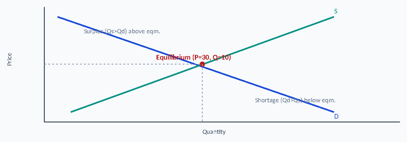
Above equilibrium (e.g. Rs.40): supply exceeds demand → surplus → price falls back. Below equilibrium (e.g. Rs.20): demand exceeds supply → shortage → price rises back. This self-correcting process is the automatic price mechanism.
Graph / Application Decision Tree
📌1) What changed – price of the good itself, or another determinant? → 2) Movement (same curve) or Shift (new curve)? → 3) Which curve is affected – D or S? → 4) Direction of shift (right = rise, left = fall)? → 5) New equilibrium price & quantity? → 6) Economic outcome / interpretation
Shifts in D & S → Effect on Equilibrium (4 Scenarios)
🔁| Scenario | Example | Curve Shift | Equilibrium Price | Equilibrium Quantity |
|---|---|---|---|---|
| Demand ↑ | Income ↑ → more chicken bought | D shifts right (D1→D2) | Rises | Rises |
| Demand ↓ | Summer→Winter → less room-cooler demand | D shifts left (D1→D2) | Falls | Falls |
| Supply ↑ | New factory → more mobile phones | S shifts right (S1→S2) | Falls | Rises |
| Supply ↓ | Input prices ↑ → fewer cars made | S shifts left (S1→S2) | Rises | Falls |
Exam clue: Demand-side shifts move Price and Quantity in the SAME direction; Supply-side shifts move Price and Quantity in OPPOSITE directions.
Market Price: Perishable vs Durable Goods
⚖️| Perishable Goods | Durable Goods | |
|---|---|---|
| Meaning | Short shelf-life, consumed quickly (dairy, fruit, vegetables) | Long life, can be stored/shelved (machinery, motorbikes, handsets) |
| Supply curve | Vertical (fixed) – supply cannot be topped up quickly once produced | Normal upward-sloping, but becomes vertical once stock is exhausted |
| Price driver | Demand side is dominant – price fluctuates mainly with demand (D1 up, D2 down) along the fixed supply | Price responds to demand within stock limits, then rises sharply once stock runs out |
Agriculture: Why Farm Prices & Incomes Fluctuate
📌Long production period + unpredictable harvest (weather, pests)
Supply curve shifts unpredictably year to year
With inelastic demand for food, price swings sharply
Ironically, when demand is elastic a good harvest can still reduce farmer income – a small price fall triggers a disproportionate rise in quantity demanded relative to revenue gained. Strong agents (e.g. big landlords, cartels) can also manipulate supply (hoarding) to distort prices for weaker producers – a key reason for government intervention.
Buffer Stock Scheme (Govt. Price Stability Policy)
🏛Mechanism: Government sets a guaranteed minimum (floor) price P1 above the free-market equilibrium P*. When supply expands (S1→S2) and would otherwise push price down to P*, the government buys up the surplus (Q1−Q2) to hold price at P1.
Objective: stable, predictable income for farmers/producers; stock can be released later if a shortage occurs.
DISADVANTAGES OF BUFFER STOCK SCHEME
- Higher opportunity cost – upfront cost of buying surplus could fund other policy goals
- Over-production risk – market price signal no longer disciplines output
- Administrative & storage costs – maintaining buffer stock is costly to run
E-business & Market Price – Key Determinants
📌BENEFITS TO FIRMS
- Lower inventory/admin cost
- Faster, cheaper marketing
- Access to global partners
BENEFITS TO CUSTOMERS
- Price comparison & better bargains
- Greater choice, reverse auctions
- Convenience/doorstep delivery
EFFECT ON PRICING
- Full info on floor prices limits over-charging
- Less brand loyalty, frequent switching
- Demand curve shifts more often
Glossary – Don't Confuse!
📖| Term | Meaning |
|---|---|
| Substitute vs Complement | Substitute = used in place of another good; Complement = used together with another good |
| Demand Schedule vs Curve | Schedule = table of price-quantity combos; Curve = graphical plot of the schedule |
| Direct vs Derived Demand | Direct = for consumer goods bought to satisfy needs directly; Derived = for capital goods/factors of production |
| Price Ceiling vs Floor | Ceiling = legal MAXIMUM price; Floor = legal MINIMUM price (govt. usually sets only one per good) |
| Giffen Good | Exception to law of demand (Robert Giffen) – as price of bread fell, real income rose enough that consumers bought LESS bread and switched to better food |
Exam Patterns & MCQ Quick Clues
🎯"Price of the good itself changes"
Movement along curve (extension/contraction)
"Income/taste/weather/population changes"
Shift of demand curve
"Input cost/technology/tax changes"
Shift of supply curve
"Qd > Qs at current price"
Shortage – price will rise
"Qs > Qd at current price"
Surplus – price will fall
⚠ ECONOMICS EXAM TRAPS
Trap: Confusing "change in demand" (shift, non-price cause) with "change in quantity demanded" (movement, price cause).
Trap: Mixing up which side dominates price for perishables (demand-driven, vertical supply) vs durables (supply matters until stock runs out).
Trap: Assuming supply and demand shifts always move price and quantity the same way – supply shifts move them in OPPOSITE directions.
Trap: Forgetting that basic necessities, Giffen goods and status goods are EXCEPTIONS to the law of demand.
Trap: Treating buffer stock's floor price as a price ceiling – it is a MINIMUM (floor), not a maximum.
PRC-3 ECONOMICS – CHAPTER 2 IN 60 SECONDS
- Demand: willing + able to buy; inverse law (income + substitution effects).
- Supply: offered for sale at a price/time; direct/positive law.
- Movement = own price change; Shift = other determinant change.
- Demand shifters: income, taste, weather, population, substitute price, ads.
- Supply shifters: input cost, technology, taxes/subsidies, price of other goods.
- Equilibrium: Qd = Qs; surplus depresses price, shortage drags it up.
- Demand shift: price & quantity move SAME way; Supply shift: OPPOSITE ways.
- Perishables: vertical supply, demand-driven price. Durables: stock-limited.
- Buffer stock: govt. floor price + buys surplus to stabilise farm income.
- E-business: more price transparency, less brand loyalty, frequent demand shifts.
Chapter Memory Map
🧠Preparing for ICAP PRC-3?
Join Learning League for chapter-wise classes, practice MCQs and tests on our student portal. Message us on WhatsApp to enrol.